The hidden costs of solar power

Solar power is the fastest growing source of electrical energy in the US. In the last year solar power generation grew by 15.52%, followed by wind at 8.27%, then natural gas at 4.17%. Solar power has captured the imagination of many as way to get unlimited “free” energy from the sun. It has been declared the cheapest and cleanest form of electrical energy by mainstream scientists and thought leaders alike.

Solar power has a much higher energy density than wind power (~7 acres/MW vs. ~60 acres/MW). This means that solar power is more suitable for constructing micro grids as there is simply no space for wind power. Micro grids are an important concept because it is becoming more difficult to get new solar and wind farms connected to the grid. The viability of industry is highly dependent on the price of energy, so it is critical to understand the real cost of a solar micro grid.

To judge solar power, four criteria will be considered: cost, reliability, CO2 emissions, and land use. The purpose of this paper is to thoroughly understand these most relevant issues.

The alleged cost of solar power

The cost of solar is currently estimated by using the levelized cost of electricity formula (LCOE).¹ The LCOE is just the cost of power generation, thus it excludes the cost of transmission, distribution, and administration. The key inputs are the overnight cost of a solar farm, operation and maintenance, interest rate, capacity factor, and life of the plant.

According to the Energy Information Agency (EIA) the overnight cost for a complete solar farm in 2023 is 1448² $/KW. The interest rate is the weighted average cost of capital (WACC). This is a combination of debt and equity. This is assumed to be 7.7%.³ This value comes from Lazard, which is a popular source for LCOE calculations. The EIA uses 6.54% as a projected WACC for 2028.

Capacity factors for states are calculated by combing two EIA sources. The first has the capacities for all of the electrical plants in the US⁴, the second has all of the annual generation data for the plants.⁵ All the values for each state are totaled in order to create an accurate weighted average capacity factor for each state. Life of a solar farm is assumed to be 30 years.

Another factor to consider is subsidies. Solar and wind power each get a 26 $/MWh federal subsidy for all the electricity they produce. This is called the production tax credit (PTC). In addition, there is an alternative subsidy of 30% of capital cost called the investment tax credit (ITC). It is a common practice that published costs of solar power factor in federal subsidies. When evaluating an energy system, it’s important to know the unsubsidized cost because subsidies don’t lower costs, they just hide them in the form of one or more of the following: higher taxes, higher debt, budget cuts, or inflation.

Table 1 shows LCOE calculations in $/MWh with various parameters. The middle column is the unsubsidized cost, using the current WACC. The right column uses the EIAs projected WACC and subtracts the PTC.

Table 1

The most accurate value for the US is $67.11. This is because it is the unsubsidized cost, using the current WACC, and using the average capacity factor for the country. The lowest number is $25.54. We get there by assuming the WACC will come down in a few years, subtracting the PTC, and using the highest statewide capacity factor, which is Nevada. The EIA estimates the cost of solar to be 23.22⁶, using 6.54% for the WACC, and 29% for the capacity factor. They are using a capacity factor that is a bit higher than Nevada. Their motive for using such a high capacity factor is unclear.

The cost of natural gas is currently about $44 MWh. MIT just released a projected, unsubsidized cost of large scale AP1000 nuclear plants at $66 MWh⁷. They calculate this number by using their open source nuclear cost estimation tool (NCET). This is a nth-of-a-kind cost projection that requires about ten AP1000s to be built in succession in order to achieve the required industrial and regulatory learning.

For an accurate comparison of nuclear to solar we need to use the nth-of-a-kind cost for nuclear. The price of solar power is currently at its nth-of-a-kind price. We know this because the price has been slowly rising in recent years, which is seen in annual EIA reports. Note, this is for the complete solar farm, not merely the solar panels

Batteries are assumed to be 250 $/KWh, 300 $/KWh including installation. This is the current price of  5 Tesla Megapacks.⁸ The cost of batteries has been fluctuating in recent years, we are currently at low point due to a battery glut in China. The efficiency of batteries is assumed to be 90%.

Influential podcaster and solar advocate David Roberts tells his listeners that the cost of solar power is in the “low twenty dollars per MWh,” and thus solar power is the cheapest form of electricity. He may be quoting from official EIA sources, but this is extremely misleading and causes policymakers to make poor decisions. For example, these low numbers appear in planning documents for northern states where the true unsubsidized LCOE is closer to the mid-eighties: New York is at 83.41 $/MWh.

However, using exaggerated LCOE calculations for estimating the cost of electricity from solar is not even close to worst intellectual offence. The LCOE of solar and wind power is virtually meaningless. This is because solar, like wind power, is a highly intermittent form of energy. To power a grid, the generated electricity must exactly match the consumer demand. This is called load balancing.

A new kind of LCOE for solar has recently emerged which includes four hours of lithium ion batteries. This is just as meaningless. It’s impossible to understand what that really means with respect to the cost of reliable electricity. What we need to know in order to make accurate policy decisions is something like: “what will the cost of electricity be to get 90% of our electricity from solar, what are the CO2 emissions, and how much land is required”. The generation system will consist of a combination of solar capacity, batteries, and gas backup that achieves this goal. No version of the LCOE will answer this kind of question.

How to study solar power

Solar power is a stochastic process which makes it impossible to understand with just a standard spreadsheet type analysis. To study solar power accurately we need a model that can perform a simulation of hourly data. The data needs two columns: the first contains the hourly consumer demand, the second contains the hourly solar production.

The EIA publishes such data for every grid region in the US.⁹ This is the combined consumer demand and solar output for the entire region, for each hour of the year, starting from mid-2018 to the present. This data can easily be normalized and rescaled to represent any specific scenario we wish to test.

A modeler was written in excel that uses a VBA function to step through each row of data. The algorithm is very simple. For each row, get the demand and solar output. If there is a surplus of energy, store it in the batteries, while accounting for storage losses. If the batteries are full, the energy is curtailed (thrown away). If there is an energy deficit, retrieve required energy from the batteries. If the batteries are empty, fill in the difference with natural gas. Two years of data are processed in this way.

The modeler is called Variational Energy Solver (VES). VES is an excel model that has enough details so we can make key predictions about costs, CO2 emissions, and land use given some specific user defined scenario. To define a scenario, VES relies on a series of key input parameters.

The two most important for studying solar power are the solar overbuild factor and hours of storage. The overbuild factor is the amount of solar power that will be generated with respect to consumer demand. An overbuild factor of 1 means that the annual solar power generated exactly equals the annual consumer demand. Generated solar power should not be confused with consumed solar power. 2 is twice the annual consumer demand. The overbuild factor ranges from 0 to infinity. The hours of storage defines the number of hours of battery storage that can satisfy 100% of consumer demand.

To answer the previously proposed question: “what will the cost of electricity be to get 90% of our electricity from solar, what are the CO2 emissions, and how much land is required”, we need to first calculate the overbuild factor and hours of storage that can power the grid such that 90% of the electricity comes from solar, at the lowest possible cost. Once we have these two values the rest of the question can be answered with simple arithmetic based on assumptions from published studies.

To calculate the overbuild factor and hours of storage VES is paired with an excel feature called Solver. Solver is a very powerful nonlinear constrained optimizer. Solver will take control of VES in order to find the ideal values of the user specified input parameters which will minimize cost, while satisfying user defined constraints.

To answer our question, the input parameters are the overbuild factor and hours of storage, the cost function to minimize is simply the cost of power, and the user defined constraint is that 90% of the consumed electricity must come from solar. By combining VES with Solver, we can now explore a vast universe of scenarios that enable us to make predictions about what will happen in real life.

The hidden cost of making solar power reliable

This section shows VES optimizations for solar power consumed at increments of 10%, starting from 0% to 100%. The baseline cost is 50 $/MWh. The baseline grid is assumed to be powered 100% by natural gas, where 95% of the gas is combined cycle, and 5% is combustion turbine. The solar data comes from the MISO grid which has a capacity factor of 24.3%. MISO is a grid region composed of several midwestern states. It was chosen because the capacity factor there is very close to the national average.

A key limitation of these results is that transmission costs as the percentage of solar power increases are not accounted for. Analyzing transmission will add severe complications and a lot of guesswork. New transmission costs will be substantial; hence the cost estimates should be viewed as lower bound estimates.

Table 2 shows the results. These are the ideal overbuild factors and hours of storage that produce the lowest possible cost for each percentage of solar power consumed.

Table 2

A common mistake that energy gurus make is to assume that the amount of solar energy required to power a grid is roughly equal to the annual electrical consumption. Notice that with an overbuild factor of 1 we only get 70% percent of our electricity from solar. 30% is lost from a combination of curtailment, storage losses, and transmission losses. Notice that the overbuild factor rises linearly until the percentage of solar consumed hits about 70%, then it begins to rise exponentially. This is depicted in Figure 1. The x axis in the following charts is the percentage of energy consumed: either solar or nuclear.

Figure 1

The optimizer does not bring in batteries until solar consumption reaches about 30%. Allowing a small amount of curtailing is cheaper than batteries at this level. At 30% batteries come in, then rise linearly until about the 90% mark, then rise exponentially.

Figure 2

Figure 3 shows the cost of power in $/MWh. This should not be confused with the retail cost which includes transmission, distribution, and administration costs. Electricity costs are often expressed in cents/KWh. To convert $/MWh to cents/KWh simply divide by 10.

Figure 3

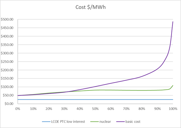
The blue line is the LCOE in Nevada, using a projected lower interest rate, and subtracting the PTC. This is the alleged cost of solar.

The green line is the projected nth-of-a-kind cost of nuclear. The optimizer brought in 2.1 hours of batteries at the 100% level. The batteries both lower the cost and help the nuclear plants follow load. The cost of nuclear bumps up near the 100% level due to the fact that it has to handle high peaks in consumer demand. If a demand shift program can flatten the highest peaks, costs for nuclear will come down significantly. This is not true for solar; VES simulations show little difference for solar when a flat consumer demand is assumed. For off grid uses by industry the cost of nuclear will stay at 66 $/MWh. This is because industrial demand is flat,

The purple line is the basic cost solar as the percentage of solar consumed increases. Note the exponential rise in the cost as the percentage increases. The fundamental error that advocates of solar (and wind) power make is that they are unaware of this exponential effect. This is because they either don’t perform hourly simulations, or their simulations are incorrectly designed.

VES predicts that cost of solar will rise to about 76 $/MWh at the 35% consumed level. Because of the PTC, consumers should not experience any significant rise in the cost of electricity at that level. This will allow advocates of solar power to boast that the use of solar power doesn’t increase electricity prices. They are blissfully unaware of the price rises to come. And the PTC will have adverse effects on the economy that won’t necessarily be correlated to the rise of solar and wind power.

The purpose of the next 3 figures is to show why there is an exponential rise in the cost of solar as the percentage increases. These figures were all produced by VES. The data is from MISO. The assumptions are that 95% of the consumed electricity comes from solar, the overbuild factor is 2.4, and the hours of storage is 23.5.

Figure 4 shows the capacity factors for each month. The highest is 33.6% for August, and the lowest is 12.1% for January. This partially explains why the overbuild factor has to be so high to make solar power reliable year round. Batteries are only useful for a few hours of storage, what is needed is months of storage. We thus have to build the system to work well in the winter. But if we build enough to work in the winter, then in the summer we get a huge surplus. This leads to huge curtailment.

Figure 4

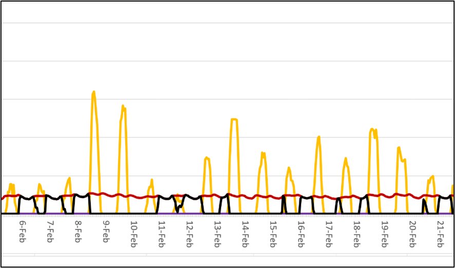
Figure 5 shows solar production in the summer at the 95% level. The yellow line is solar, the red line is consumption. The solar peaks are significantly higher than the consumption peaks due to the high overbuild factor. This is causing a large amount of curtailment.

Figure 5

Figure 6 shows that in the winter, even with an overbuild factor of 2.4, and 23.5 hours of batteries, gas is still needed to avoid blackouts. Gas is the black line. Notice that at night gas often supplies all of the consumer demand. This shows that even at 95% solar, all of the gas capacity must be ready to step in and power the grid. Therefore, the fixed costs of gas do not fall unless solar can fully power the grid.

Figure 6

To fully power the grid without gas, the overbuild factor and hours of storage will have to nearly double from here, as can be seen from table 2, yet we get only an additional 5% solar consumed.

The hidden cost of CO2 emissions

The whole purpose of solar power is to reduce CO2 emissions; thus, it must be judged on this basis. There is an implicit assumption that X% of solar power consumed reduces CO2 emissions by X%. But this is not the case, we therefore must make a cost correction.

For example, let’s say that we get 40% of our electricity from solar. We naturally assume that CO2 emissions fall by 40%. But after a deep life cycle assessment (LCA), we discover CO2 emissions only fell by 20%. We effectively got half the solar power we paid for. This is equivalent to saying the real cost of solar power is double what we thought it was.

The following formula is used to correct for this:

    C-cost = B-cost / (Actual reduction / Expected reduction)

Where:

    C-cost is the cost adjusted for hidden CO2 emissions

    B-cost is the basic cost of power described in the previous section

    Expected reduction is the percentage of solar consumed

    Actual reduction is the actual CO2 reduction computed using an LCA

There are several reasons why CO2 emissions don’t fall as much as is expected: CO2 emitted from the cradle to grave production of solar farms, CO2 emitted from the cradle to grave production of batteries, extra CO2 emissions from combined cycle gas plants (or coal plants)  due to fast ramping, and the excessive use of lower efficiency gas plants for load balancing intermittent energy.

The National Renewable Energy Laboratory (NREL) published (2024) a detailed report on the cradle to grave CO2 emissions for a complete solar farm.¹⁰ Their median estimate is 930 kg-CO2/KW, installed in the US. This assumes polysilicon panels, single-axis tracker, 0.7% degradation rate, and a 30 year system life. The scope of the assessment includes mining, production, installation, maintenance, and recycling. This does not include batteries.

For batteries we assume 90 kg-CO2/KWh. This is based on a cradle to gate analysis, assuming batteries are manufactured in China.¹¹ This is a comprehensive study; however, it’s for car batteries. There doesn’t seem to be a high quality study yet for grid batteries. Ideally, we would like an assessment of Tesla megapacks since they are the batteries assumed in this study.

When a grid has a high percentage of intermittent energy, the fossil fuel resources have to do more work in order to load balance, this will be called fast ramping. A combined cycle plant produces the least amount of CO2 emissions when it runs at full power: 337.7 kg-CO2/MWh. As it reduces its power CO2 emissions rise. At 30% of full power emissions are 459 kg-CO2/MWh.¹² The intermittent nature of solar power causes gas (and coal) plants to reduce their output more than they would otherwise have to in order to load balance. VES computes the total amount of solar power used directly by consumers (unbuffered by batteries). This is the amount of gas energy affected by having to load balance solar; thus, this is the fast ramping portion of the gas. VES adds 10% more CO2 emissions to the fast ramping portion of the gas energy. This is a lower bound estimate.

When a grid has a high percentage of intermittent energy, there may be a tendency to use more combustion turbines to load balance as opposed to using combined cycle plants. The reason is that a combustion turbine is more flexible. It can operate from 0% to 100% of its power range, whereas a combined cycle plant is generally limited to operating from 40% to 100% of its power range. In addition, a combustion turbine generator can be much smaller than a combined cycle plant. Therefore, a solar powered microgrid will likely use a gas powered combustion turbine as the backup energy. The problem is that combustion turbines emit 50% more CO2 than combined cycle plants. This must be considered when comparing a microgrid to a large-scaled grid. VES has an option to assume all gas backup comes from a combustion turbine. This option is important to model microgrids accurately.

Table 3 shows the results of the CO2 adjustments.

Table 3

The numbers from the 3rd column are the CO2 emissions. The costs from the 4th column come from the previous section. The costs from the 5th column are cost adjusted for hidden CO2 emissions. Figure 7 below adds the graph of the CO2 adjusted emissions (in red) to the previous graph.

Figure 7

Notice that in column 3 the CO2 emissions start to rise beyond the 95% level. This is due to the excessive overbuilding and batteries required to get to higher levels of reliability. This is shown in figure 8.

Figure 8

The baseline emissions are 466 gr-CO2/KWh. At the 100% level emissions fall by only 79%. If we do a minimization for CO2 emissions, the lowest achievable is 87.8 gr-CO2/KWh at the 95.5% level. This results in an 81.17% reduction in CO2 emissions.

Let’s now consider a microgrid where 75% of the electricity comes from solar. A large scale grid can use a highly efficient combined cycle plant for the gas backup, however, the microgrid will have to use a smaller less efficient generator. Assuming a flat demand curve (for industrial uses), and efficiency of the generator is 40%. The CO2 reductions are only 57%, not the 75% reductions implied. The basic unsubsidized cost is 150.3 $/MWh, and the CO2 adjusted cost is 197.2 $/MWh - about 4 times greater than the baseline. The CO2 emissions are about 200 gr-CO2/KWh. This a long way from a CO2 free solution. Attempting to go higher than 75% will result in steep cost increases and smaller CO2 reductions.

The hidden cost of manufacturing solar power

In the previous sections we assumed that solar power was manufactured with fossil fuel energy. This prevents us from completely eliminating CO2 emissions. In this section we assume that solar power and batteries are manufactured from the output of solar power, stabilized by batteries. This could achieve the goal of zero emissions, but at a higher price. The reason costs will go up is because significantly more energy produced by the grid will have to be reinvested back into building the grid when it is powered by solar vs fossil fuel.

We start with a concept called energy returned on energy invested (ERoEI).¹³ ERoEI is defined by the following ratio:

    ERoEI = (energy delivered) / (energy required to deliver that energy)

A healthy grid has an ERoEI greater than 10. As the ERoEI decreases toward 1 the grid gets sicker. If the ERoEI equals 1, then all the energy produced is equal to the energy needed to produce it, thus there is no energy available for general consumption. We could say there is an energy black hole where the event horizon is ERoEI equal to 1. In this section we will use the ERoEI to make predictions on how much costs will have to rise in order to achieve genuine zero emissions for current electrical consumption.

In the literature, estimates for the ERoEI of solar power range from .82 to greater than 30. This seems to indicate that an accurate ERoEI is impossible to calculate, but the wild variations are mostly due to disagreements on how to interpret it. The lowest number assumes an electrical grid in northern Europe and includes virtually everything required to make the energy reliable. This is called the extended ERoEI.¹⁴ A middle of the road estimate, recommended by NREL, is 9-10.¹⁵ This is for a complete solar farm, but no storage or other external factors. The highest estimates use a modified ERoEI formula which gives solar power extra credit for displacing inefficient coal plants.

To calculate a useful ERoEI we need to include all the energy inputs needed to modify the grid we are modeling. Consider the following equation:

    E = C/(S + B + T)

Where:

    E is the ERoEI

    C is the energy delivered to consumers

    S is the energy needed to create solar farms

    B is the energy needed to create batteries

    T is the energy needed to create new transmission

C is simply the annual consumer demand. For the US this is about 4,000,000 GWh. To calculate the energy inputs, we need two categories of information: the energy needed to make each component, and the quantity of each component needed to achieve some specified percentage of solar consumed.

The energy needed to make each component is called the cumulative energy demand (CED). We get the CEDs from published research. For solar farms we use the average CED from the previously cited NREL study: 12,000 MJ/KWdc.¹⁶ For batteries we use a meta study of car batteries: 328 KWh/KWh¹⁷. Note, for batteries we need the storage capacity as opposed to the charge/discharge capacity. Ideally, we would like the CED for Tesla megapacks, or something similar, but that is not available. Grid batteries are typically heavier with more electronics vs car batteries. There are apparently no high quality studies estimating the CED for transmission, thus we use 0. This is in keeping with the philosophy that it is better to underestimate costs rather than overestimate.

VES will calculate the quantities of solar capacity and batteries needed to achieve the specified percentage of solar consumed. This means that the ERoEI is highly dependent on the percentage of solar consumed. It will start high and go lower as the percentage increases.

The ERoEI cited by NREL is useless. Using it is similar to using the LCOE for pricing solar. Everything depends on the percentage of solar consumed! If VES computes an ERoEI using the same philosophy the NREL study uses, the number is about 12. This is where the numerator is the total energy created by a solar farm and the denominator is the CED of that solar farm (no batteries).

Fossil fuel resources are intentionally omitted from this ERoEI calculation. The reason is because that energy has already been paid for. If we were building a fossil fuel grid for the first time, we would need to include them. Our goal here is to predict the cost of changing the grid we currently have in order to achieve some specified percentage of solar consumed. The fossil fuel resources will be gradually phased out. This means that the baseline ERoEI is infinity.

We will now use the ERoEI to calculate the resources needed to make solar power from solar power. To do this we have to use it to derive a variable called the resource multiplier (RM). RM is then used to adjust the quantity of each component in the grid.

    RM = 1 + 1/(ERoEI – 1)

    SC_T = SC*RM

    BC_T = BC*RM

    T_T = T*RM

    C_T = C*RM

SC, BC, TC are the solar, battery, and transmission capacities needed to provide the current consumer demand - C. SC_T, BC_T, and TC_T are the solar, battery, and transmission capacities needed to provide both the consumer demand, and the new demand needed to make solar, batteries, and transmission. C_T is the energy needed to serve consumers plus the energy needed to make solar, batteries, and transmission.

Below is a derivation of RM. For those who dislike math, no worries, skip the derivation as there will be no future references to it.

Begin Derivation of RM

we start with the ERoEI equation:

    E = C/I₀

E is the ERoEI, C is the energy delivered to consumers, and I₀ is amount of energy needed to make the solar required to produce C. I₀ does not include the energy needed to make itself.

Rearrange:

    I₀ = C/E

Since I₀ is the energy to make new solar, we now have to calculate the energy to make it as well. This is equal to I₀/E. I is the total amount of energy needed to make energy:

    I ≈ I₀ + I₀/E

To make I exact we must continue this process forever:

    I = I₀ + I₀/E + (I₀ /E)/E + …

Substitute C/E for I₀ and factor:

    I = C (1/E + 1/E² + 1/E³ + …)

The infinite series (1/E + 1/E² + 1/E³ + …) converges to:

    1/(E – 1)

Substitute into previous equation:

    I = C/(E – 1)

We have to add this to the original C to get the total energy needed for general consumers and the builders of solar, batteries, and transmission:

    C_T = C  + C/(E - 1)

Factor and substitute:

    C_T = C(1 + 1/(E – 1))

    RM = 1 + 1/(E – 1)

    C_T = C*RM

End Derivation of RM

When ERoEI is infinity, RM is 1. When ERoEI is 1, RM is infinity. Figure 9 shows the relationship.

Figure 9

Table 4 shows the results with ERoEI adjustments.

Table 4

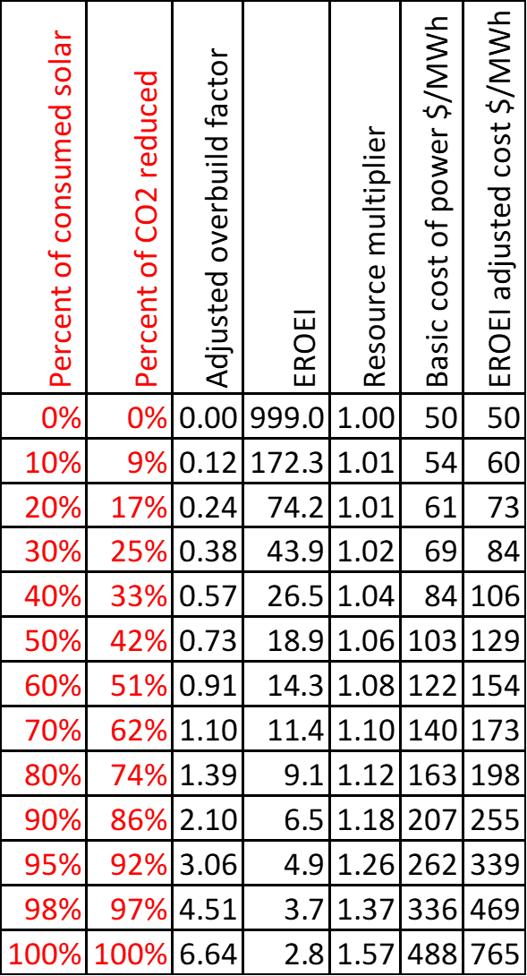
Column 2 is the CO2 emissions reduced when the solar is made from solar. Column 5 is the RM for the percentage of solar consumed. Column 3 is the adjusted overbuild factor, which is the basic overbuild factor from table 2 times column 5. Column 6 is the basic cost of solar from table 2. Column 7 is the cost of solar power when the solar power is made by solar power and adjusted for hidden CO2 emissions.

Figure 10

Figure 10 adds the graph of the ERoEI adjustments to figure 3. Blue is the alleged cost of solar. Purple is the basic cost of solar. Black is the ERoEI adjusted cost from column 7. Green is the cost of nuclear. Estimates of the ERoEI for a nuclear plant range from 25 to 75. The ERoEI of a grid powered by nuclear will come down slightly due to a small amount of overbuilding and batteries, but the RM will be near 1, thus the ERoEI effects are irrelevant.

The hidden land use

A typical calculation for land use involves computing the amount of solar power that generates the same amount of electricity equal to the annual electrical consumption. This ignores intermittencies, seasonal fluctuations, and CO2 emissions not from generating electricity.

L = C/(365*24*CF)*7*1000

Where L is the land use in acres, C is the annual consumer demand in GWh, 365*24 is the number days in the year, CF is the average capacity factor of the US, 7 is the acres/MW of a solar farm, and 1000 converts GWh to MWh.

4,000,000/(365*24*.243)*7*1000 = 13,318,112 acres

This is .66% of the lower 48 states. Not so bad if this were true. This is for a grid with an overbuild factor of 1. Table 2 shows us that even with 12 hours of batteries such a grid will provide power no more than 70% of the time, with only a 61% reduction of CO2 as seen in table 3.

If the current grid is completely decarbonized that will reduce CO2 emissions by about 31%. To get to true net zero requires substantially more electricity. This includes new electricity for charging EVs, electric trucks, heat pumps, making steel, solar modules, batteries, concrete, fertilizer, plastics, chemicals, paper, data centers, etc. In addition, we need to make synthetic fuel for plugin hybrids, tractors, ships, large trucks, trains, the military, planes, and jets. Let’s assume it requires at least 3 times the current electrical consumption to electrify these applications. This will be called the grid expansion factor (EF).

Total land use = 13,318,112 *OF*RM*EF

Where:

OF = overbuild factor

RM = resource multiplier

EF = grid expansion factor

For 100% solar consumed, and zero emissions, we get OF from table 2, RM from table 4, and EF = 3.

L = 13,318,112*4.21*1.57*3

   = 264,086,174 acres

This is 13.2% of the lower 48 states. This is for true net zero, excluding transmission and mines.

The hidden cost of transmission

The transmission we have today was designed to carry electricity from reliable power plants to load centers. Reliability here means electricity on demand with a high capacity factor: coal, gas, hydroelectric, and nuclear. Power plants are located as close as possible to load centers to keep transmission costs down. The US transmission has just over 700,000 miles of high voltage power lines and 46,000 substations (not counting line taps). If we had to build it today the overnight cost would be about 2 trillion dollars.

Using the current transmission to transmit intermittent power, with a low power density, and a low capacity factor poses serious challenges that are not widely understood. There are two major problems that are essential to understand.

The first is that solar (and wind) farms will have to be much further from load centers than traditional power plants. The reason is because there is simply not enough space near any high voltage power lines to put them. The best spots have been taken. It now takes on average 5 years to get a connection to the grid, up from under 2 years in 2008¹⁸. Building a spider web of new high voltage power lines to vast rural areas is going to be very expensive, disruptive, and there is currently no mechanism to fund it. Apparently, the authors of the IRA had only a superficial understanding of how renewable energy works as it subsidizes solar and wind power, but very little for new transmission.

The second is that the transmission lacks the transmit capacity needed to handle the large power spikes that will come as the amount of solar (or wind) power increases. To see this let’s consider a very simple example. Suppose we have two choices to power our city: either nuclear or solar. Assume we need 1000 MW for peak consumption, the capacity factor of the nuclear is 100% (it’s really only 92.5%), and for solar it’s 25%.

In the nuclear option we only need to transmit at most 1000 MW of power. In the solar option we need to transmit up to 4000 MW of power. This is because with a capacity  factor of 25%, we must fluctuate between 0 and 4000 to get the average of 1000. When percentages of solar power are low there is often enough excess capacity to transmit power spikes, but this will change as the amount of solar power increases. Texas currently curtails about 10% of their solar power due to congestion, and California curtails about 4% due to congestion.

There are two solutions to this problem. The first is to rebuild the transmission with higher volage power lines and substations. This will cost several trillion dollars and cause massive disruption. The second is to collocate batteries with solar farms in order to turn them into reliable power. This option is easier to do but it comes at a severe cost that is not understood.

If we turn each solar and wind farm into a reliable plant with overbuilding and batteries as discussed in previous sections, we will prevent the energies from widely distributed solar and wind farms from mixing their energy. That means there will be no complimentary effects. For instance, weather conditions in location A are favorable (excellent sun or wind), in B they are poor, but combined we get a more acceptable average. The summer is best for solar but worst for wind. Winter is the worst for solar, but decent for wind. By mixing the energies prior to storage and consumption we get less curtailing and thus need less overbuilding and storage.

Energy models, including this one, typically assume that the grid is capable of full energy mixing. This is because the data sets are the combined energies for a whole region as opposed to individual solar or wind farms. This assumption also makes the models much easier to build. But these models don’t account for the cost of building a transmission capable of full mixing. Since this model is for solar power only, the results should be fairly accurate because solar farms within one grid region have a high degree of correlation. But there will still be some complementary effects from mixing solar, so the costs described in previous sections should be viewed as lower bound estimates.

Some very influential models are fatally flawed. For example, Mark Jacobson’s model¹⁹ assumes perfect mixing for all solar and wind farms for the entire US: “This study has many uncertainties. One is the assumption of a perfectly interconnected transmission system in each region.” He claims costs are accounted for but provides no details. Imagine a grid that is like a giant sheet of copper covering the entire US. To build such a grid, each of the AC grid regions will have to be rebuilt with higher voltage AC lines and substations, and a new national grid of HVDC power lines will have to be built to connect the AC sub grids. The cost of a single HVDC substation is nearly a billion dollars, and each HVDC power line needs at least 2 of them.

The costs and disruptions of building this kind of grid are astronomical. And there are no plans to build such a grid. Policy makers (and academics) don’t seem to understand that such a grid is necessary for their grand vision. Without such a grid (and even with), Jacobson‘s results are meaningless. Mark Jacobson is one of the most influential advocates of solar and wind power in the world. Politicians base their energy plans in part on his claims. Also beware of models that have exotic features like making hydrogen with curtailed solar, then storing it in large underground caverns. These models likely depend on this kind of super-grid.

There are no complimentary effects when mixing solar with nuclear. While it is theoretically possible for nuclear to load balance solar or wind, it makes no economic sense. This can be seen by looking at figure 6. For nuclear power to backup solar (or wind) there has to be enough nuclear capacity to power the entire grid during long streaks of poor solar. This means that the only savings possible is for the variable cost of nuclear. But the variable cost of nuclear is only about 10% of the total annual costs, this a fraction of the cost of the solar. Thus, it’s always significantly cheaper to go with 100% nuclear than any combination of solar and nuclear. This is true regardless of how powerful the transmission is.

Conclusion

A metaphor that describes the results of this paper is as follows: imagine there are two roads that lead to the same destination - a place called net zero. One of the roads is named solar road, the other is named nuclear road.

Solar road starts out fairly smooth. There are a lot of bumps, a few potholes, but it seems like progress is being made to the destination. Almost a third of the way, the road turns muddy, vehicles are getting dirty, and progress is slowing. At about the halfway point, travelers have to start using 4 wheel drive, driving is extremely unpleasant, and they are burning a lot more gas than they thought they would. Just beyond the halfway point they start getting hopelessly stuck in mud.

Some will travel further down this road than others. California will go further due to its wealth, lack of heavy industry, sunny weather, and political alignment. Most will turn around a lot sooner. Climate mitigation is meaningless if only a few wealthy regions do it.

Nuclear road is the opposite experience. The road starts out very muddy and unpleasant. There’s a lot of fear that the road is impassable, but the maps say it’s a good road, so the enlightened travelers proceed. As they travel down the road it begins to dry out and travel gets easier. Soon it becomes paved and they quicky get to their destination.

Reality is consistent with VES’s predictions. Germany shut down all of their nuclear plants and now they get 43.9% of their electricity from solar and wind²⁰, CO2 emissions are 284 gr/KWh, and the retail price of electricity is 40 cents/KWh.²¹

France gets 67.1% of its electricity from nuclear and 14.4% from hydroelectric²², CO2 emissions are 37 gr/KWh, and the retail price of electricity is 28 cents/KWh.²³ France’s CO2 emissions are even lower than the emissions of grid powered 100% by solar when an LCA is considered. For Germany to reduce CO2 emissions anywhere near as low as France’s, by building a lot more solar and wind, electricity prices will go substantially higher yet due to the exponential effects discussed previously.

The irony is that France wasn’t even trying lower CO2 emissions, they just wanted a secure source of affordable energy.

---

1. https://www.nrel.gov/analysis/tech-lcoe-documentation.html

2. https://www.eia.gov/outlooks/aeo/assumptions/pdf/elec_cost_perf.pdf

3. https://www.lazard.com/research-insights/levelized-cost-of-energyplus

4. https://atlas.eia.gov/datasets/eia::power-plants/explore

5. https://www.eia.gov/electricity/data/eia923

6. https://www.eia.gov/outlooks/aeo/electricity_generation/pdf/AEO2023_LCOE_report.pdf

7. https://web.mit.edu/kshirvan/www/research/ANP201%20TR%20CANES.pdf

8. https://www.tesla.com/megapack

9. https://www.eia.gov/electricity/gridmonitor/dashboard/electric_overview/US48/US48

10. https://www.nrel.gov/docs/fy24osti/87372.pdf

11. https://www.sciencedirect.com/science/article/pii/S0959652624011739

12. https://www.frontiersin.org/journals/energy-research/articles/10.3389/fenrg.2020.00151/full

13. https://en.wikipedia.org/wiki/Energy_return_on_investment

14. https://www.sciencedirect.com/science/article/pii/S0301421516301379

15. https://www.nrel.gov/docs/fy17osti/67901.pdf

16. https://www.nrel.gov/docs/fy24osti/87372.pdf

17. https://www.mdpi.com/2313-0105/5/2/48

18. https://emp.lbl.gov/sites/default/files/2024-04/Queued%20Up%202024%20Edition_1.pdf

19. https://web.stanford.edu/group/efmh/jacobson/Articles/I/145Country/22-145Countries.pdf

20. https://lowcarbonpower.org/region/Germany

21. https://www.statista.com/statistics/263492/electricity-prices-in-selected-countries

22. https://lowcarbonpower.org/region/France

23. https://www.statista.com/statistics/263492/electricity-prices-in-selected-countries