
Even if solar panels and batteries are free, solar power is still unaffordable

Advocates of solar power frequently remind the critics that the cost of solar modules and batteries has declined sharply over the past decades. These costs have indeed come down; see Figures 1 and 2.


Figure 1 shows that the wholesale price for solar modules is now well below $500/kWdc. Figure 2 shows that the price of lithium-ion battery cells has fallen by about 80% in the last 10 years to $78/kWh.
These remarkable cost reductions have led to the claim that solar power is now the cheapest form of electricity and may become even cheaper. However, this claim does not account for the fact that most of the costs of a solar farm are not due to the cost of battery cells and solar modules. In this paper, we will assume that solar panels and battery cells are free. We will then see how this assumption affects the expected real-life cost of a grid powered by solar energy.
The initial focus will be on solar power because of the recent interest in solar powered micro grids to power industry, and because solar power is seen as more scalable than wind power. The focus will then broaden into a discussion of mixing solar and wind in highly optimized proportions. This discussion will focus on the work of Mark Z Jacobson.
Jacobson, a Stanford professor, is the world’s most influential advocate for renewable energy. Leaders in the US and globally rely on his findings to guide their plans for transitioning to 100% renewable energy. In his 2022 paper1, he claims that the US can produce electricity using 100% Wind, Water, and Solar (WWS) for 8.66 cents/kWh (86.6 $/MWh). This figure is significantly lower than the current price of electricity. We will shed light on this remarkable claim.
How to study the cost of intermittent energy
This paper extends my previous research, 'The Hidden Cost of Solar Power,’2 which examines solar energy's major hidden costs. Here, we focus on the basic cost using the latest EIA pricing data, assuming battery cells and solar panels are free. For other interesting topics on hidden costs, refer to 'The Hidden Cost of Solar Power.'
Lazard and the EIA estimate solar power costs using the Levelized Cost of Energy (LCOE). However, LCOE is not meaningful for weather-dependent energy because to make it reliable requires overbuilding, batteries, underutilized fossil fuel backup, and transmission upgrades. The LCOE does not account for these extra costs. Adding X hours of battery storage to the LCOE does not improve the meaning.
A useful way to understand the cost of intermittent energy will answer a question such as: “what is the cost of powering a grid when 80% of the consumed electricity comes from solar power and the rest comes from gas”. If we can answer this question accurately for every percentage of solar power consumed, we can then predict the true cost of solar power given some specific policy milestone. Policy makers will then have a useful tool for accurate policy making.
To estimate the cost of intermittent energy I developed a tool called Variational Energy Solver (VES). VES uses data published by the EIA that shows the hourly consumer demand and production of electricity for all the types of electrical generators in the US.3 In addition, it has a data set for each grid region. VES rescales this data to simulate various scenarios of electrical capacity and storage.
VES is written in Excel and uses VBA functions to perform the simulations. The simulation algorithm is very simple. VES steps through each line of data trying to satisfy consumer demand with the intermittent power available for that hour. If there is a surplus, the surplus is stored. If there is a deficit, the energy required to satisfy demand is retrieved from storage. If demand still cannot be met, gas is used. The transmission and battery losses are accounted for (7% and 10% respectively).
VES relies on key driving variables to define a specific scenario. Three examples include the overbuild factor, hours of storage, and percentage of intermittent energy that is solar. The value of the driving variables determines the capacity of resources deployed, which in turn determines the cost.
An overbuild factor of 1 means annual intermittent energy production equals demand. An overbuild factor of 2 means production is twice the demand. The overbuild factor ranges from zero to infinity. Hours of storage indicate how long batteries alone can meet demand. The percentage of solar energy specifies the percentage of intermittent energy that is solar, the rest is wind. Solar power uses single-axis tracking, and wind power is onshore.
VES is paired with Solver, Excel’s constrained optimizer. Solver enables users to select multiple driving variables, such as the overbuild factor, hours of storage, and percentage of intermittent energy that is solar. Users then define a variable to minimize, for example, the cost of power. Finally, any number of constraints can be selected, such as the percentage of intermittent energy consumed.
Solver will then control VES to adjust the driving variables to find the lowest price for powering a grid with a specified percentage of consumption coming from intermittent energy, while the remainder is powered by gas. We can now estimate costs for any combination of solar, wind, and gas power in any grid region in the US. From the description above, anyone with basic Excel and programming skills can reproduce the results in this paper.

The cost of battery storage
There are misconceptions about the nature of the battery storage needed to load balance intermittent energy. Advocates of intermittent energy often confuse battery packs or cells (figure 2) with Battery Energy Storage Systems (BESS). To store surplus energy from solar or wind farms, a BESS is required. A fully installed BESS is substantially more than a collection of battery cells in a pack.
The EIA publishes detailed annual reports on the capital costs of various types of energy systems. These reports are a collaboration between the EIA and the private sector to produce accurate overnight capital cost estimates. This paper uses the latest report (2024).4
Figure 3 below is a breakdown of the individual cost components of a BESS. Two changes were made from the EIA report: costs are converted to $/kWh, and item 1 was added. The cell cost comes from figure 2. The EIA report estimates the cost of a BESS unit is $253/kWh. It does not list the cost of the cells. Item 2 is the cost of the BESS unit minus the cost of the cells.

The BESS has to send power to the grid in the correct voltage and frequency, without significant fluctuations. It must charge when energy is available (or prices are low) and discharge the correct amount of power when energy is needed. It has to remain cool and operate within parameters to ensure a long life. Installing a BESS involves acquiring permits, planning, civil works, and connections to the grid.
The major components of the BESS unit are the Battery Module, Battery Management System, Power Conversion System, Energy Management System, Thermal Management System, Communication and Control Systems, Enclosures and Safety Systems, and Monitoring and Diagnostics Tools.
Item number 4, balance-of-plant, includes auxiliary power equipment and transfer switches, inverters, medium-voltage transformers, cabling and conduit, equipment foundations, and supervisory control and data acquisition (SCADA).
The non-battery cell costs of a BESS include mature items like cables, inverters, transformers, air conditioners, sub-station, switch yard, engineering labor, and manual labor. There is no reason to believe these costs will fall. In fact, they can easily go higher. If the cost of battery cells falls to zero, the overall cost of a BESS will fall from $436/kWh to $358/kWh, an 18% reduction.
In Jacobson’s 2022 paper, he predicts the cost of storage will drop to $60/kWh by 2035. It’s not clear what he means by storage. The word BESS does not appear in his paper. He describes storage as “$60/kWh-electricity storage”. It appears as though he is only accounting for the cost of the cells. While battery cells might drop to $60/KWh, this will only lower the cost of a BESS from $436/kWh to $418/kWh, a 4% reduction.
There are plausible alternatives to lithium-ion storage, but it is important to carefully analyze the costs. For example, sodium-ion battery cells are estimated to be 25% cheaper. If these are used instead, the cost of a BESS will drop by about 4%, assuming the rest of the BESS is similar. However, sodium-ion batteries are reportedly less efficient than lithium-ion batteries. An absolute reduction in efficiency greater than 4% will increase the effective cost of a BESS, despite the decrease in the cost of the cells.
The cost of a solar farm
The argument in this section follows the same reasoning as the previous section. The cost of solar modules is only about a third of the cost of a fully installed solar farm. Data for this section comes from the same EIA report as the previous section. Note that prices are in AC for modules, as opposed to DC in Figure 1. AC prices are higher due to the common practice of oversizing the DC capacity to achieve higher inverter utilization. Figure 4 below lists the individual cost items in a solar farm.

The components of a solar farm include modules, cables, single-axis trackers, racks, combiner boxes, inverters, transformers, civil works, connections to a water source (for cleaning), control systems, switchyards, connections to the grid, acquiring permits, environmental impact study, land, engineering labor, and manual labor.
The non-module costs are for mature items, and there is no reason to believe that these costs will fall. They can just as easily rise. For example, the cost of transformers has been rising significantly in recent years. In addition, there will be pressure to switch to more advanced (and expensive) inverters to help resolve voltage and frequency stabilization issues. If the cost of solar modules were to fall to zero, the cost of a solar farm would fall from $1502/kWac to $1021/kWac, a 33% reduction.
According to the EIA report, solar power prices are no longer falling, “As solar modeling and engineering software advances, projects are able to optimize layouts and ground coverage for the lowest levelized cost of energy; however, in recent years, this only serves to limit the cost increases rather than to cause a material decrease in total project costs.”
Jacobson's 2022 paper predicts solar PV costs will fall to $775/kW, about half the current price, and assumes a solar farm lifespan of 48.5 years compared to EIA’s 35 years. Additionally, he estimates wind power at $1020/kW, while the EIA places it at $1489/kW. Onshore wind power costs have remained stable at around $1500/kW for years, with manufacturers struggling to make profits. There is no evidence to suggest prices will fall, prices can easily go higher. In fact, NREL has wind at about $2,000/kW.
Cost of solar power
The data for the results of the optimizations in this section are from the MISO grid region. MISO is composed of several states in the Midwest of the US. MISO was chosen because its solar capacity factor matches the national average (24.7%); hence, some states will do better, some will do worse. MISO is thus a good proxy for the nation. Two years of data were simulated. Intermittent energy is set to 100% solar, hence the driving variables are overbuild factor, and hours of storage.
Figure 5 shows the results of the optimizations. The first column is the percentage of solar power consumed, with the remaining power coming from natural gas. The second column shows the expected CO2 reductions compared to 100% natural gas. There are many reasons why the CO2 reductions are less than expected. This subject is discussed in detail in 'The Hidden Cost of Solar Power.' The third column presents the most accurate cost of power for each percentage of solar power consumed. The fourth column shows the cost of power assuming batteries and solar modules are free. These costs do not include distribution and administration costs.

In a 100% solar-powered grid, if batteries and solar panels are free, the cost falls from $586/MWh to $458/MWh, a 22% reduction. However, $458/MWh is approximately ten times more expensive than the current cost of power. Therefore, solar power remains unaffordable even with free batteries and solar panels.
In addition, 100% solar power is only about a 75% reduction in CO2 emissions because manufacturing solar modules and batteries is done with fossil fuel. To achieve genuine zero emissions, batteries and solar panels must be made with the output of solar energy, and this will drive up costs even more due to solar power’s low energy returned on energy invested (EROEI). This topic is covered in detail in ‘The hidden cost of solar power.’
According to this MIT study5, the projected nth-of-a-kind (NOAK) Levelized Cost of Electricity (LCOE) of nuclear power is $66/MWh. We are interested in NOAK cost because this is the future cost if nuclear power is built at scale, as opposed to Lazard, which relies heavily on the cost of the last build. To meet peak demand, the optimizer chose a nuclear overbuild factor of 1.4 and 1.2 hours of battery storage. The batteries help lower costs and facilitate load balancing. When 100% of power consumption is met with nuclear energy, the cost is $103.4/MWh.
Figure 6 shows the costs in graph form. Blue is the alleged cost of solar power. This is EIA’s LCOE minus the federal Production Tax Credit (PTC). Green is the projected NOAK cost of nuclear power. Red is the cost of solar power, assuming batteries and solar panels are free. Purple is the most realistic cost of solar power, assuming batteries and solar panels are manufactured with fossil fuel.

Why solar power is so expensive
The next five figures tell the story of why solar energy is so expensive. Figure 7 and 8 shows the output of solar power in the summer and winter, respectively. Yellow is solar power, red is demand, and black is gas.


In this scenario there is enough solar power to meet consumer demand for 98% of the year. The optimizer recommends a 3.5 overbuild factor and 19.2 hours of storage. In the summer we will have a large surplus, which leads to large curtailment. In the winter, demand must be met with 100% gas during cold nights, even with 19 hours of storage.
Having a reliable solar-powered grid with no gas will require significantly more solar capacity and storage, with only a small increase in solar energy consumed. This leads to an exponential growth rate in costs. Until 100% is achieved, all of the gas capacity must be available to meet consumer demand. This means two parallel energy systems must be maintained.
Figures 9 and 10 show the optimized values for the driving variables as the percentage of solar power consumed increases. Figure 11 shows the rise in curtailment.
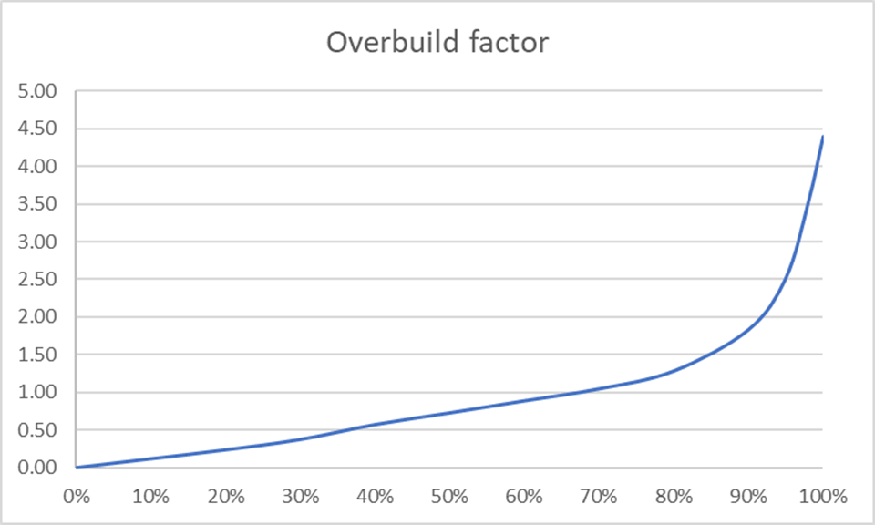
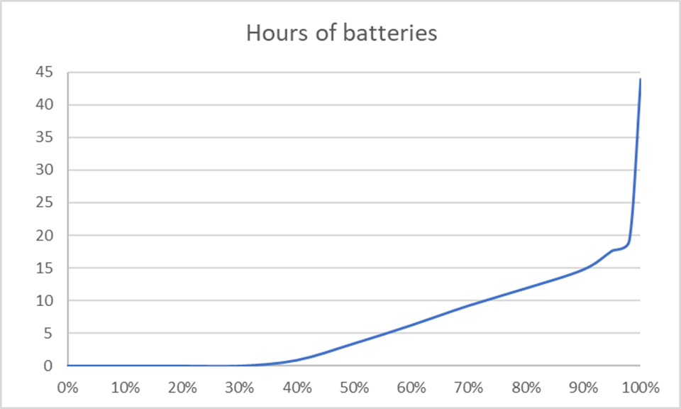
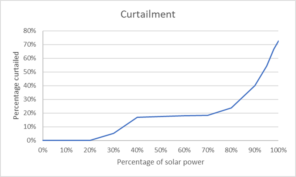
The cost increase of solar power can be divided into three phases: honeymoon, linear, and exponential. The honeymoon phase spans from 0% to 30% usage, where costs rise from $49.6/MWh to $70.5/MWh. This increase is offset by the Production Tax Credit (PTC). However, the PTC must be financed by other means, thus the cost is merely shifted. At 30%, no batteries are needed, and curtailment is only about 5%.
The linear phase spans from 30% to 70%. Costs rise linearly from $70.5/MWh to $161/MWh, batteries usage is increasing, and curtailment is steady at around 18%. Consumers will begin to see significant increases in prices despite the PTC. Industry will be under economic pressure and many will be uncompetitive.
The exponential phase spans from 70% to 100%. Costs, capacity, battery usage, and curtailment all rise exponentially. Costs rise from 161/MWh to 586/MWh. Consumers will be under extreme stress and industry will be uncompetitive.
The super grid
The discussion so far is only about solar power. Understanding 100% solar power is important because, in many regions, solar power is more scalable than wind power, and micro grids will likely be 100% solar-powered due to land limitations. However, many of the renewable energy plans such as Mark Jacobson’s call for a mix of solar and wind power.
In principle, combining solar and wind power can reduce the cost of each alone by exploiting their complementary effects. In summer, solar power is at its highest, while wind is at its lowest. In winter, solar is at its lowest, while wind is at its average. Combining the two reduces seasonal volatility.
Mixing energy from wind farms at different locations also exploits complementary effects. Location A may have good wind output while location B has poor output. On a different day, it can be the other way around. Mixing the energies from the two locations produces a more reliable output. The larger the region of combined energy, the smoother the output is. However, exploiting these complementary effects at scale will require rebuilding the electricity grid.
Powering a grid with a high percentage of intermittent energy will require two kinds of grid upgrades. First, solar and wind plants have a low energy density. This means they will have to be located in rural areas where there is enough space. As a result, power lines will need to be extended to connect all of these highly dispersed plants to the main grid. Building new power lines is very expensive and politically difficult. Developers are running out of spots near high voltage transmission lines, and this is causing a slowdown in building new plants.
The second type of upgrade is to increase the voltage of the power lines to exploit the complementary effects that can be achieved by mixing intermittent energy sources into a common electricity pool. Batteries are then located near load centers, far away from the solar and wind farms. Final load balancing is done mostly with batteries just prior to the electricity entering into the distribution (lower voltage lines in the city).
The current grid was designed to transmit power from dispatchable plants to load centers. The voltage of each power line is chosen to be able to handle the peak load, about 1.6 times the annual average. The goal was to use the lowest possible voltage because higher voltage lines are more expensive and disturb more land. Therefore, transmitting power higher than 1.6 times the average load can overload the line.
The current grid is not compatible with high percentages of intermittent energy because the power output from a solar or wind farm fluctuates from 0 to (overbuild factor)/(capacity factor). For example, with a solar capacity factor of 0.25 and an overbuild factor of 2, we need to transmit power up to 8 times the average load to avoid curtailing and exploit complementary effects (2/0.25). However, exceeding a factor of 1.6 can overload the line.
At low percentages of intermittent energy, this is not a problem. For example, let’s say the overbuild factor is .4 and the capacity factor is .25. In this case, we would only have to transmit 1.6 times the average load (.4/.25). No problem – the grid was designed for that. However, as the overbuild factor rises above .4, the grid will become more congested, and excess power will have to be curtailed. Another feature of the honeymoon phase is that complementary effects can be exploited without grid upgrades because the overbuild factor does not rise above about .4.
In states with high percentages of intermittent energy, like Texas and California, grids have become congested when weather is favorable, and they are forced to curtail excesses. The chosen solution is to co-locate batteries with the solar and wind farms. A power spike is then sent to the battery instead of the grid. The battery then transmits lower amounts of power to the grid over a longer period of time. The intermittent plants now act more like dispatchable plants.
This solution works fine, but now there will be no complementary effects! This important point seems to have been lost. Without complementary effects, a region might as well build 100% of what works best for that region. So, California would build only solar power, and Iowa only wind power. This is another reason it’s useful to study just 100% solar power. We can do a separate study on 100% wind power. That would be very useful for states in the wind belt such as Iowa.
To achieve significant complementary effects, the grid will need to be rebuilt, which will be extremely disruptive and expensive. Power lines, towers, and substations will need to be replaced with larger, more costly versions. Additionally, transmission corridors must be widened, leading to substantial eminent domain issues. This upgraded infrastructure will be referred to as a "super grid." Considering the challenges posed by NIMBYism (Not In My Backyard) when building a single power line, it is hard to imagine the public supporting a complete rebuilding of the grid.
The most important aspect of Jacobson’s plan is his reliance on a grid so efficient that it allows for perfect mixing across regions the size of the US – like a giant sheet of copper covering the whole country. Here is a quote from his paper, “This study has many uncertainties. One is the assumption of a perfectly-interconnected transmission system in each region.” He divides the world into 20 regions, with the US being one of them.
Jacobson does not account for the cost of building a grid capable of achieving this level of "perfect" connectivity. He is not alone in this oversight; many models make the mistake of assuming perfect connectivity within a grid region without considering the cost of the necessary grid upgrades.
The existing grid has about 700,000 miles of high voltage transmission lines and about 45,000 substations, excluding line taps. It is composed of many regional sub-grids, such as MISO. The voltage levels range from 90kv to 765kv, with 138kv being the most common, and less than 1% are 765kv. If constructed today, the current grid would cost around 2 trillion dollars.
To create a regional AC super grid, such as for MISO, the power lines and substations will need upgrading to significantly higher voltages. Most of the lines will need to be raised from 138kV to the 345kV to 765kV range. In this case, there will be high connectivity within each regional grid but not for the country as a whole. This will easily cost more than double the cost of the current grid. Consider the cost of a double circuit 138kV line is $2.7 million per mile, and a 345kV line is $5.3 million per mile.6The corresponding increase in substations is also about double. The cited price guide doesn’t list double circuit lines higher than 345kV; hence, the cost of two single circuit 500kV lines is $4 million per mile each.
Building a national super grid will cost significantly more than a regional super grid. This is because it will require a large number of long-distance HVDC power lines and DC substations to connect the regional super grids into a perfectly interconnected whole. We cannot replace all of the nation’s AC lines with HVDC lines because the cost of a single DC substation is almost a billion dollars. Recall there are about 45,000 substations. Note that the Inflation Reduction Act only allocates $2.9 billion for all grid upgrades. Oops.
It’s all about the grid
In this section we will evaluate four views of load balancing:
Load balance a single solar or wind farm.
Load balance a regional AC super grid.
Load balance a national AC/DC super grid with reasonable inputs.
Load balance a national AC/DC super grid with Jacobson’s inputs.
Load balancing a single plant is the most difficult because there are no complementary effects. Load balancing a regional super grid is easier because complementary effects arise from mixing all the energy within the grid region. Load balancing a national super grid is the easiest because all the energy in the nation is mixed. The larger the area, the more effective the complementary effects are, the easier it is to load balance. In this section, the data has a capacity factor of 24.7% for solar power and 35% for wind, as these are national averages.
Modeling a single plant predicts the cost when batteries are co-located with the plant. By using overbuilding and batteries, we turn a single intermittent plant into a dispatchable one. Modeling a single solar or wind farm is more difficult than modeling a super grid. By using EIA data, we are assuming a super grid because the data represents the total for all the plants in the region.
The EIA does not have data for individual plants. To model a solar or wind farm, we first get hourly solar irradiance and wind speed data from NASA’s power project. It allows us to select from any point on Earth. To convert the solar irradiance data into solar farm output, VES uses the HDRK model. For wind power, VES uses power curves for commonly used windmills. VES continues to use the EIA’s consumer demand data.
Figure 12 shows the assumptions Jacobson uses in his 2022 paper. Jacobson does not mention interest rates in his paper. So, in keeping with his trend of optimistic assumptions, we will use 5%.

Jacobson relies on a complex demand response program. VES will simply allow a 2% failure rate and assume that a demand response program will work to prevent blackouts. By doing it this way, we don’t have to be concerned about the details of how a demand response program works; we are only interested in the savings. This is then compared to the cost of a 0% failure rate, where no demand response is assumed.
In a world powered 98% by solar and wind, failure typically happens during winter nights, although it can occur in all four seasons. It’s not clear that any form of demand response can eliminate blackouts without having a gas backup system ready to step in. Consider Figure 13 below. We assume a regional super grid in MISO. We also assume there is enough intermittent energy to power the grid 98% of the time. The optimizer chose a mix of 40.5% for solar power and 59.5% wind. Here, the wind almost disappeared for three days in the winter when there was very little solar (blue represents wind power). It’s hard to imagine how any demand response program could handle a case like this. Not even rolling blackouts will work for this case.

Figure 14 assumes a national super grid, with 98% of electricity coming from intermittent energy sources. In this scenario, the optimizer chose 24.8% solar and 75.2% wind. Although the situation has improved, demand will still need to be cut by about 50% for an entire winter night to achieve load balance without gas. With a 98% reliability rate, failures will occur frequently throughout the year. Therefore, a demand response program could be very painful for consumers, even if it is feasible. Going to a 1% failure rate will reduce the burden of the demand response program, but costs will rise dramatically due to the exponential effects previously discussed.

Figure 15 shows the results of 9 VES optimizations. Column 8 shows the cost of power in $/MWh. This does not include the cost of distribution, and administration. Jacobson’s cost analysis does include these items. VES assumes the pre-solar and wind era cost of power plus transmission is $49.6/MWh, and the cost of distribution and administration is $57/MWh. Recalling his estimate for the cost of electricity was $86.6/MWh, we will subtract $57/MWh to get $29.6/MWh for his estimate of the cost of only power.
Column 9 shows how the cost of power estimates affects electricity prices. The increase is calculated by subtracting the baseline cost of power ($49.6/MWh) from the cost of the power estimate, then dividing the result by 10 to convert to kWh. This provides an estimated increase in the cost of electricity in cents per kWh for industrial, commercial, or retail consumers – all are affected equally by the rise in the cost of power. This cost does NOT include the cost of building the super grid. To account for this, a back-of-the-envelope calculation suggests adding an additional 15 to 30 cents/kWh to the cost of cases 5 to 9.

Cases 1 through 4 represent the typical cost of power from individual solar and wind farms. This is the scenario when we use the current grid with batteries co-located with the plants. These plants now behave like dispatchable plants, making them compatible with the current grid. The cost is about 10 times the current cost of power, even when allowing for a 2% failure rate. Note the cost of solar power is higher than in previous sections because we were using EIA data which assumes a super grid. However, the difference is not that great because the complementary effects in a 100% solar powered grid are fairly small.
Cases 5 and 6 assume a regional super grid for MISO. In general, the optimizer prefers wind power over solar, but at ultra-high percentages, wind power can sometimes become more expensive. This is because in a grid region like MISO, it has a more severe worst-case scenario. Recall that in the 2 years of MISO data simulated, wind can disappear for three days. Allowing a 2% failure rate makes a big difference because the less common but most severe cases can be ignored. However, the cost of power is still four times more expensive, plus the cost of building a regional super grid.
Cases 7 and 8 assume a national super grid. To simulate this, we simply use the EIA’s national data set. With reasonable assumptions, the cost of power comes down to $315/MWh. Allowing a 2% failure rate cuts the cost to $147/MWh. However, even with a painful demand response program, power is still three times more expensive, plus the cost of building a national super grid.
In case 9, we assume a national super grid with Jacobson’s assumptions from figure 12. The cost of power comes down to $54/MWh. Although not quite as low as his $29.6/MWh, power at this price would be comparable to the current price of power.
Conclusion
The cost of solar modules and battery cells constitutes a small percentage of the total cost of solar energy at scale. While the prices have decreased significantly over the years, further reductions will have minimal impact. The other costs, being mature items at NOAK prices, are likely to fluctuate based on market conditions. There is no reason to expect these costs will fall, they can just as easily rise. These other costs, due to the overbuilding needed for reliability, are the primary reason why intermittent energy is so expensive.
This paper began with an analysis of 100% solar power, then diverged into a discussion about the grid. This divergence was essential because critics could plausibly claim that 100% solar power is a strawman. After all, influential models rely heavily on the complementary effects of mixing solar and wind power. These complementary effects are real, but to achieve them, the grid must be rebuilt. However, these models fail to discuss the need for a grid capable of exploiting complementary effects, the cost of building it, and the disruptions it will cause.
Energy models that do not acknowledge these issues are invalid! Without complementary effects, regions may as well use 100% of what works best for their region. This brings us back to where we started. It looks like most regions are now preferring solar power over wind. Since there are no plans to rebuild the grid (or funding), they may as well use 100% solar power.
It is clear that the current trend in storage is to couple batteries with solar and wind farms in order to reduce grid congestion. Reconductoring the grid with newer materials, at great cost, might help some, but this just delays the day of reckoning. To achieve the results predicted by models, it will require raising the voltage of the lines and substations. Reconductoring the grid seems like a waste of money.
The cheapest way to power a large country like the US with only solar and wind power is to build a national super grid and then implement a severe demand response program. It’s not clear that building such a grid is even possible, either politically or technically. In addition, it is not clear that the public will accept the kind of demand response program that can avoid the worst case scenarios without maintaining a parallel fossil fuel backup. If both of these could be done, VES estimates the cost of power will be $147/MWh. Including the cost of the super grid will easily double this. In spite of the added cost of the grid, this approach is cheaper than the alternatives. The total estimated increase in cost over current rates, including building the super grid, is about 25 to 40 cents/kWh.
In contrast, using MIT’s NOAK estimate for nuclear power and optimized levels of overbuilding and storage, a nuclear-powered grid will add about 5.4 cents/kWh to the current cost of electricity, with no need for a demand response program or the disruptions of rebuilding the electricity grid. The MIT study does not consider regulatory reform, so further reductions are possible with strong political leadership.7
By using Jacobson’s assumptions, VES was able to come fairly close to reproducing his results. Jacobson uses a variety of other resources, such as pumped-hydro, not considered by VES, but by assuming his low estimate for lithium-ion storage, they are not relevant. Therefore, the critical discrepancy is not in how Jacobson simulates compared to VES, but in his optimistic assumptions listed in Figure 12, his assumption of 'perfect' connectivity for the entire US, not accounting for the costs of building a grid capable of providing this, and his elaborate demand response program.
Excellent! Given the incessant claims about how "easy" and "cheap" it would be to convert to 100% Ruinable energy, your article elucidates many reasons why the real world data demonstrates that intermittent energy is incredibly expensive. Nonetheless, the academic zealot promoters will continue the politically approved narratives.
Meanwhile...
All time world record consumption of natural gas in 2024.
All time world record consumption of oil in 2024.
All time world record consumption of coal in 2024.
The modern world was built by, and is sustained by, the products and energies of hydrocarbons. All historical data demonstrates that all energies are cumulative and additive, not substitutes. The world burns more than 2x more wood today than it did a century ago.
IMHO, the world will consume more hydrocarbons 50 years from now than it does today. Hydrocarbons are miracle resources.
https://www.visualcapitalist.com/visualizing-the-scale-of-global-fossil-fuel-production/
Good read! Love the invention of Variable Energy Solver (VES). I worked in rooftop solar for 13 years and often mused that the cost of the panels would become free, and that our work was still so challenging to integrate custom houses, often having to upgrade service panels, roofs, trees and even the architecture of the home in order to get a decent yield and a place to property house the energy storage systems. Transitioned my career to nuclear three years ago and haven't looked back.